We’ll follow along with the example used in Chapter 3 of Mostly Harmless. You can download the 1980 census from https://economics.mit.edu/faculty/angrist/data1/data/angkru95. Load the data along with tidyverse().
library(tidyverse)
library(R.utils) #for file path (you may not need this)
library(AER)
library(texreg) #for nice tables
library(sandwich)
library(estimatr)
library(lfe)
census <- read_delim(filePath(path,"asciiqob.txt"),
delim = " ",
col_names = c("lwklywge","educ","yob","qob","pob"),
n_max = 329509)
# remove extra spaces using stringr package
# and convert to numeric from character
census <- census %>%
mutate(lwklywge = as.numeric(str_trim(lwklywge, side = "left")),
educ = as.numeric(str_trim(educ, side = "left")),
yob = as.numeric(str_trim(yob, side = "left")),
qob = as.numeric(str_trim(qob, side = "left")),
pob = as.numeric(str_trim(pob, side = "left")))
# create variable that is year and quarter of birth
census$yqob <- as.numeric(paste0(census$yob,".",census$qob))
# average weekly wage
avg <- census %>%
group_by(yqob) %>%
summarize(avg_wkwg = mean(lwklywge),
avg_educ = mean(educ))Average education by quarter of birth
ggplot(data = avg, aes(x = yqob, y = avg_educ)) +
  geom_point() +
  geom_line() +
  ggtitle("Average Education by Quater of Birth (First Stage)") +
  xlab("Year of Birth") +
  ylab("Years of Education") +
  theme_bw()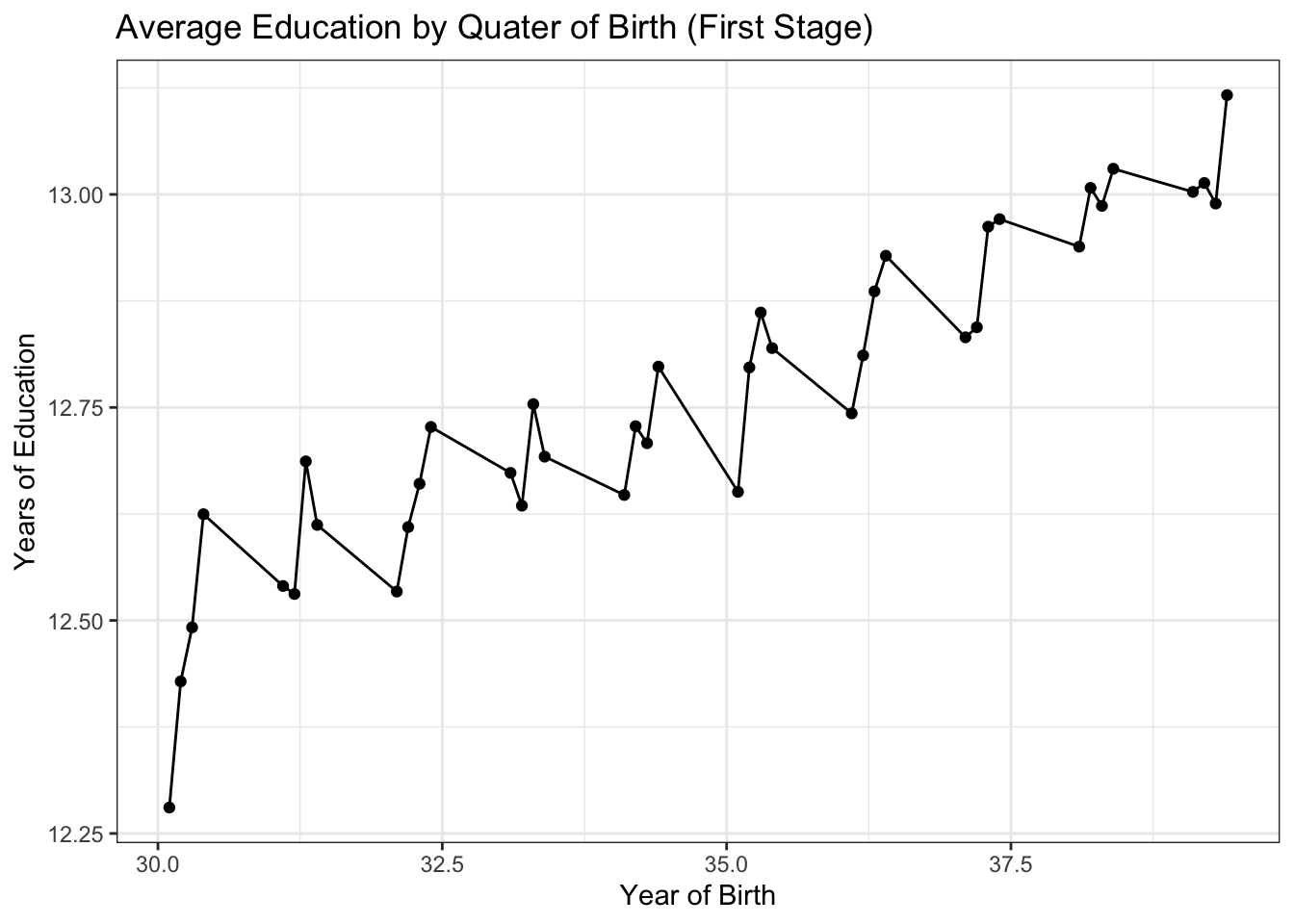
Average weekly wage by quarter of birth
ggplot(data = avg, aes(x = yqob, y = avg_wkwg)) +
  geom_point() +
  geom_line() +
  ggtitle("Average Weekly Wage by Quartter of Birth (Reduced Form)") +
  xlab("Year of Birth") +
  ylab("Log Weekly Earnings") +
  theme_bw()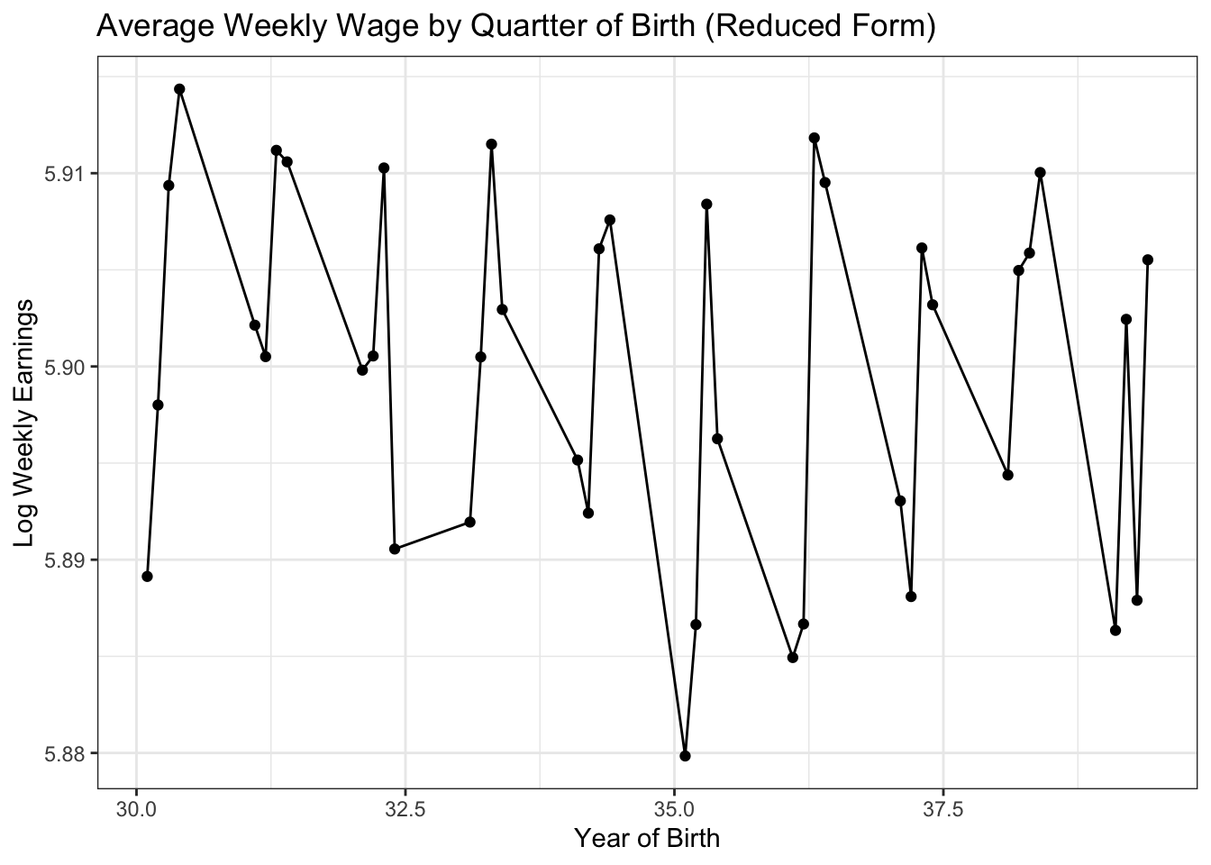
OLS estimation
ols <- lm(lwklywge ~ educ, data = census)
ols_robust <- lm_robust(lwklywge ~ educ, data = census, se_type = "HC1",ci=FALSE)
coeftest(ols, vcov=vcovHC, method="HC1")
##
## t test of coefficients:
##
## Estimate Std. Error t value Pr(>|t|)
## (Intercept) 4.99518232 0.00507394 984.48 < 2.2e-16 ***
## educ 0.07085104 0.00038103 185.95 < 2.2e-16 ***
## ---
## Signif. codes: 0 '***' 0.001 '**' 0.01 '*' 0.05 '.' 0.1 ' ' 1sqrt(vcovHC(ols, type = "HC1")) #to compare SEs## Warning in sqrt(vcovHC(ols, type = "HC1")): NaNs produced## (Intercept) educ
## (Intercept) 0.005073871 NaN
## educ NaN 0.0003810234summary(ols)##
## Call:
## lm(formula = lwklywge ~ educ, data = census)
##
## Residuals:
## Min 1Q Median 3Q Max
## -8.7540 -0.2367 0.0726 0.3318 4.6357
##
## Coefficients:
## Estimate Std. Error t value Pr(>|t|)
## (Intercept) 4.9951823 0.0044644 1118.9 <2e-16 ***
## educ 0.0708510 0.0003386 209.2 <2e-16 ***
## ---
## Signif. codes: 0 '***' 0.001 '**' 0.01 '*' 0.05 '.' 0.1 ' ' 1
##
## Residual standard error: 0.6378 on 329507 degrees of freedom
## Multiple R-squared: 0.1173, Adjusted R-squared: 0.1173
## F-statistic: 4.378e+04 on 1 and 329507 DF, p-value: < 2.2e-16summary(ols_robust)##
## Call:
## lm_robust(formula = lwklywge ~ educ, data = census, se_type = "HC1",
## ci = FALSE)
##
## Standard error type: HC1
##
## Coefficients:
## Estimate Std. Error t value Pr(>|t|) CI Lower CI Upper DF
## (Intercept) 4.99518 0.005074 NA NA NA NA NA
## educ 0.07085 0.000381 NA NA NA NA NA
##
## Multiple R-squared: 0.1173 , Adjusted R-squared: 0.1173
## F-statistic: 3.458e+04 on 1 and 329507 DF, p-value: < 2.2e-162SLS estimation
## dummy for QOB == 1
census$q1 <- ifelse(census$qob==1,1,0)
iv <- ivreg(lwklywge ~ educ | q1, data = census)
htmlreg(list(ols,iv),doctype = F, digits=3,custom.model.names = c("OLS","IV"))| OLS | IV | |
|---|---|---|
| (Intercept) | 4.995*** | 4.597*** |
| (0.004) | (0.306) | |
| educ | 0.071*** | 0.102*** |
| (0.000) | (0.024) | |
| R2 | 0.117 | 0.095 |
| Adj. R2 | 0.117 | 0.095 |
| Num. obs. | 329509 | 329509 |
| ***p < 0.001; **p < 0.01; *p < 0.05 | ||
Looking at the Inclusion Restriction
Is our instrument highly correlated with the endogenous regressor? We manually run the first stage and make sure to correct our standard errors for possible heteroscedasticity.
iv_stage1 <- lm(educ ~ q1, data = census)
coeftest(iv_stage1, vcov = vcovHC, type = "HC1")
##
## t test of coefficients:
##
## Estimate Std. Error t value Pr(>|t|)
## (Intercept) 12.7968834 0.0065712 1947.433 < 2.2e-16 ***
## q1 -0.1088179 0.0133159 -8.172 3.043e-16 ***
## ---
## Signif. codes: 0 '***' 0.001 '**' 0.01 '*' 0.05 '.' 0.1 ' ' 1# we could compare to results using the lfe package
test <- felm(lwklywge ~ 1 | 0 |(educ ~ q1)| 0,data=census)
#summary(test$stage1)$coefficientsContinue to estimate 2SLS using the predicted values from the first stage.
census$educ_pred <- iv_stage1$fitted.values
tsls <- lm(lwklywge ~ educ_pred, data = census)
coeftest(tsls,vcov=sandwich)
##
## t test of coefficients:
##
## Estimate Std. Error t value Pr(>|t|)
## (Intercept) 4.597477 0.322077 14.274 < 2.2e-16 ***
## educ_pred 0.101995 0.025221 4.044 5.255e-05 ***
## ---
## Signif. codes: 0 '***' 0.001 '**' 0.01 '*' 0.05 '.' 0.1 ' ' 1coeftest(iv, vcov=sandwich)##
## t test of coefficients:
##
## Estimate Std. Error t value Pr(>|t|)
## (Intercept) 4.597477 0.306889 14.9809 < 2.2e-16 ***
## educ 0.101995 0.024032 4.2442 2.194e-05 ***
## ---
## Signif. codes: 0 '***' 0.001 '**' 0.01 '*' 0.05 '.' 0.1 ' ' 1Compare results between using the AER package and doing 2SLS by hand. We should see that the coefficients are the same but the standard errors are different.
iv_se_robust <- coeftest(iv, vcov=sandwich)[,"Std. Error"]
tsls_se_robust <- coeftest(tsls, vcov=sandwich)[,"Std. Error"]
htmlreg(list(iv,tsls),
        custom.model.names = c("ivreg","by hand"),
        doctype = F,
        override.se = list(iv_se_robust,tsls_se_robust),
        digits = 3)
## Warning in override(models = models, override.coef = override.coef, override.se
## = override.se, : Standard errors were provided using 'override.se', but p-values
## were not replaced!| ivreg | by hand | |
|---|---|---|
| (Intercept) | 4.597*** | 4.597*** |
| (0.307) | (0.322) | |
| educ | 0.102*** | |
| (0.024) | ||
| educ_pred | 0.102*** | |
| (0.025) | ||
| R2 | 0.095 | 0.000 |
| Adj. R2 | 0.095 | 0.000 |
| Num. obs. | 329509 | 329509 |
| ***p < 0.001; **p < 0.01; *p < 0.05 | ||