Nonparametric Regression
Given the usual conditional expectation function
\[E[y_i | \mathbf{x_i} = \mathbf{x}] = m(x)\]
we can estimate \(m(x)\) as a traditional linear model or nonparametrically. One approach to nonparametric estimation is to use a binned means estimator. This takes the average \(y\) for some values of \(x_i\) close to \(x\) (assuming \(x_i\) is continuous). In other words, take the average \(y_i\) for all values \(x_i\) where \(|x_i - x| \leq h\) for some small \(h\). Here \(h\) is the bandwidth.
Binned means estimator
\[\begin{equation} \widehat{m}(x) = \frac{\sum_{i=1}^n \mathbb{1}(|x_i - x| \leq h)y_i}{\sum_{i=1}^n \mathbb{1}(|x_i - x|\leq h)} \end{equation}\]
This gives us a step-function because the indicator function makes the weights discontinuous. Alternatively, we can replace the indicator function with a kernel function:
Kernel regression estimator
\[\begin{equation} \widehat{m}_k(x) = \frac{\sum_{i=1}^n K\left(\frac{x_i - x}{h}\right)y_i}{\sum_{i=1}^n K\left(\frac{x_i - x}{h}\right)} \end{equation}\]
Some commonly used kernels:
Gaussian Kernel: \[K(u) = \frac{1}{\sqrt{2 \pi}} exp \left (-\frac{u^2}{2}\right)\]
Epanechnikov Kernel: \[ K(u) = \left\{ \begin{array}{ll} \frac{3}{4\sqrt{5}}\left(1 - \frac{u^2}{5}\right) & \mbox{if $|u| < \sqrt{5}$}\\ 0 & \mbox{otherwise}\end{array} \right. \]
Local Linear approximation
Let’s start with simulating some data using the simstudy packge:
library(tidyverse)
## simulate data using simstudy package
library(simstudy)
set.seed(234)
df <- genData(100, defData(varname = "x", formula = "20;60", dist = 'uniform'))
theta1 = c(0.1, 0.8, 0.6, 0.4, 0.6, 0.9, 0.9)
knots <- c(0.25, 0.5, 0.75)
df <- genSpline(dt = df, newvar = "y",
                predictor = "x",
                theta = theta1,
                knots = knots,
                degree = 3,
                newrange = "90;160",
                noise.var = 64)
Here is a scatterplot with dashed vertical lines showing the knots used to generate the data (quantiles).
## scatter plot of the data
ggplot(data = df, aes(x = x, y = y)) +
  geom_point() +
  geom_vline(xintercept = quantile(df$x, knots), linetype = 'dashed') +
  theme_bw()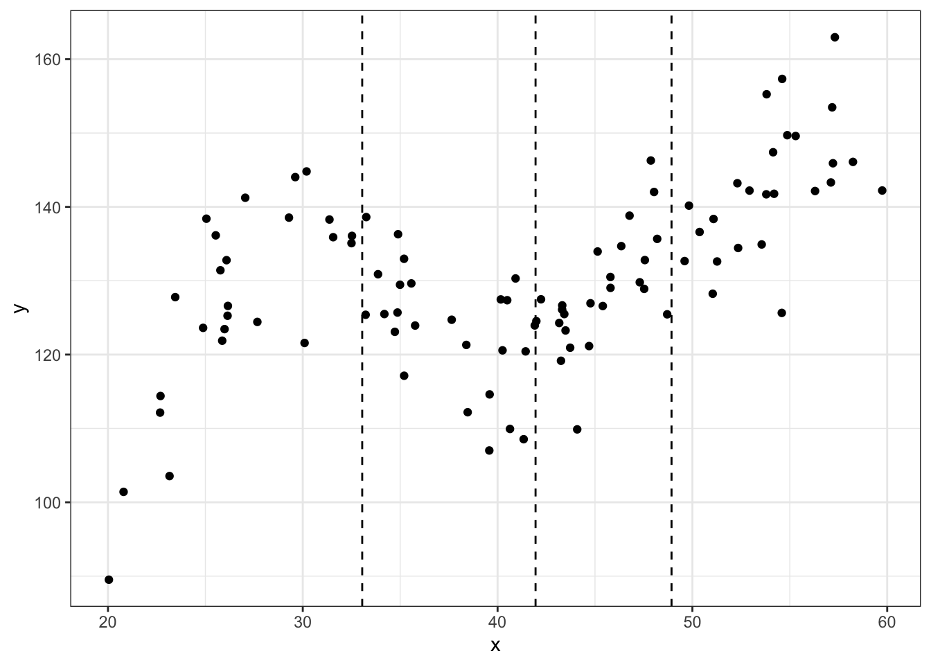
#using locpoly
library(KernSmooth)
## KernSmooth 2.23 loaded
## Copyright M. P. Wand 1997-2009m_ll <- data.frame(locpoly(df$x, df$y, degree = 1, bandwidth = 3))
# degree = 1 for locally linear
ggplot(data = df, aes(x = x, y = y)) +
geom_point() +
geom_vline(xintercept = quantile(df$x, knots), linetype = 'dashed') +
geom_line(data = m_ll,aes(x = x, y = y),color = "blue") +
theme_bw()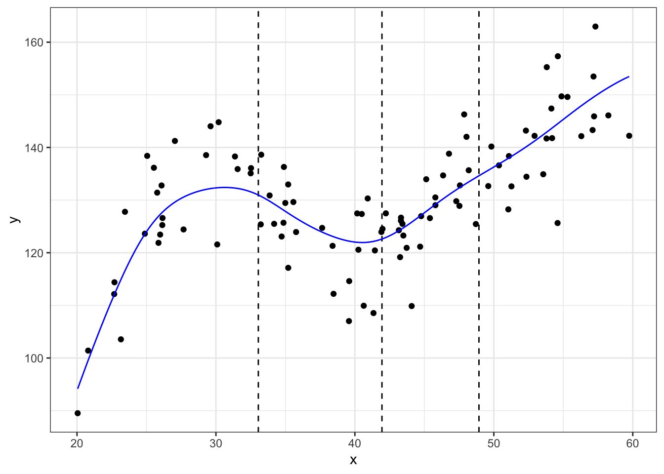
tricube kernal \[ K(u) = \left\{ \begin{array}{ll} (1-|u|^3)^3 & \mbox{for $|u| < 1$}\\ 0 & \mbox{for $|u|\geq 1$ }\end{array} \right. \]
kernel.function <- function(u){
  tmp <- rep(NA,length(u))
  for(i in 1:length(u)){
    if(abs(u[i])<1){
    k <- (1 - abs(u[i])^3)^3
  }else if(abs(u[i])>=1){
    k <- 0
  }
    tmp[i] <- k
  }
  return(tmp)
}
Decide on evaluation points \(x_0\). Our data is (roughly) from 20 to 60 so let’s use that to define our evaluation points and we will use increments of 20.
# evaluation points
x0 <- seq(25,55,10)
# bandwidth
h <- 10
We have 3 evaluation points, let’s do a loop to calculate the scaled distance from each value of \(x\) to \(x_0\).
# empty container
distances <- matrix(NA, nrow = length(df$x), ncol = 4)
colnames(distances) <- x0
for(i in 1:length(x0)){
  # calc distance and put in column i
  distances[,i] <- df$x - x0[i]
  # divide by sum of bandwidth (this does scaling)
  # want scaled so can use as weights
  #distances[,i] <- distances[,i]/sum(distances[,i])
}
Now apply our kernel function to estimate the weights
distances <- data.frame(distances)
weights <- map_df(distances, kernel.function)
Estimate predicted values at the evaluation points using our weights
# eval point 20
W_25 <- diag(weights$X25)
X <- as.matrix(cbind(rep(1,100), df$x)) #create X matrix with intercept
Y <- as.matrix(df$y)
B_WLS_25 <- solve(t(X)%*%W_25%*%X)%*%(t(X)%*%W_25%*%Y)
# eval point 40
W_45 <- diag(weights$X45)
B_WLS_45 <- solve(t(X)%*%W_45%*%X)%*%(t(X)%*%W_45%*%Y)
# eval point 60
W_55 <- diag(weights$X55)
B_WLS_55 <- solve(t(X)%*%W_55%*%X)%*%(t(X)%*%W_55%*%Y)

# predicted values
yhat <- data.frame(y25 = X%*%B_WLS_25,
                   y45 = X%*%B_WLS_45,
                   y55 = X%*%B_WLS_55)
yhat <- pivot_longer(yhat, names_to = "group", names_prefix = "y",
                     values_to="yhat",cols = c(1:3))

df_big <- bind_cols(bind_rows(df,df,df),yhat)
#first eval point
ggplot(data = df_big %>% filter(group==25), aes(x = x, y = y)) +
  geom_point() +
  geom_point(aes(x = x, y = yhat),color="red") +
  theme_bw()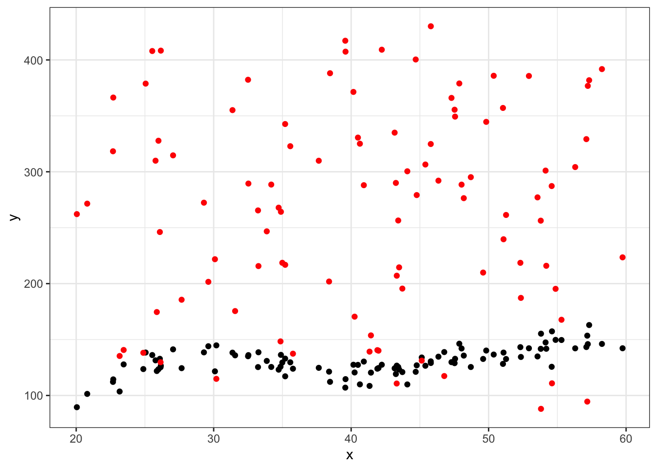
ggplot(data = df_big %>% filter(group==45), aes(x = x, y = y)) +
  geom_point() +
  geom_point(aes(x = x, y = yhat), color="green") +
  theme_bw()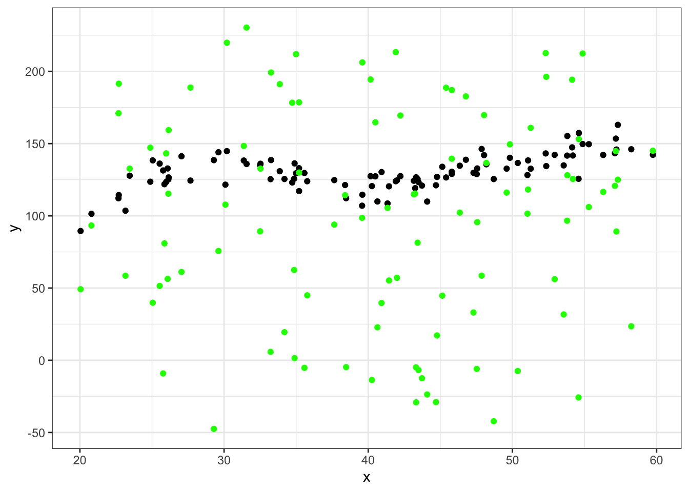
ggplot(data = df_big %>% filter(group==60), aes(x = x, y = y)) +
  geom_point() +
  geom_point(aes(x = x, y = yhat), color="blue") +
  theme_bw()
ggplot(data = df_big, aes(x = x, y = y)) +
  geom_point() +
  geom_point(aes(x = x, y = yhat, color=group)) +
  theme_bw()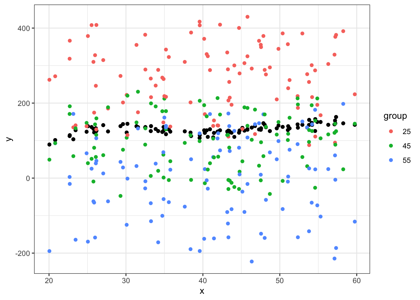
Switching gears – let’s do a quick example on how to demean variables using dplyr. We will use the built-in mtcars dataset.
First, let’s demean only one column, the mpg column and make a new variable using mutate():
df <- mtcars %>%
  mutate(mpg_demean = mpg - mean(mpg))
You have to assign this to an object, in this case I’ve stored it as an entirely new data.frame df. I can now use this new variable:
head(df$mpg_demean)## [1] 0.909375 0.909375 2.709375 1.309375 -1.390625 -1.990625Here, the demeaned variable is calculated but not stored because I have not assigned this operation to anything. If I try to call the variable mpg_demean later I will get an error because it does not exist.
mtcars %>%
  mutate(mpg_demean2 = mpg - mean(mpg)) %>%
  head()
## mpg cyl disp hp drat wt qsec vs am gear carb mpg_demean2
## 1 21.0 6 160 110 3.90 2.620 16.46 0 1 4 4 0.909375
## 2 21.0 6 160 110 3.90 2.875 17.02 0 1 4 4 0.909375
## 3 22.8 4 108 93 3.85 2.320 18.61 1 1 4 1 2.709375
## 4 21.4 6 258 110 3.08 3.215 19.44 1 0 3 1 1.309375
## 5 18.7 8 360 175 3.15 3.440 17.02 0 0 3 2 -1.390625
## 6 18.1 6 225 105 2.76 3.460 20.22 1 0 3 1 -1.990625head(df$mpg_demean2)## NULLIf I want to de-mean multiple variables at once use mutate_each. Here I am selecting two columns, vs and am, then using mutate_all to demean them both then I’m joining them back to the original data.
df <- df %>%
  select(vs, am) %>%
  mutate_all(list(~. - mean(.))) %>%
  bind_cols(df,.)
## New names:
## * vs -> vs...8
## * am -> am...9
## * vs -> vs...13
## * am -> am...14head(df)## mpg cyl disp hp drat wt qsec vs...8 am...9 gear carb mpg_demean vs...13
## 1 21.0 6 160 110 3.90 2.620 16.46 0 1 4 4 0.909375 -0.4375
## 2 21.0 6 160 110 3.90 2.875 17.02 0 1 4 4 0.909375 -0.4375
## 3 22.8 4 108 93 3.85 2.320 18.61 1 1 4 1 2.709375 0.5625
## 4 21.4 6 258 110 3.08 3.215 19.44 1 0 3 1 1.309375 0.5625
## 5 18.7 8 360 175 3.15 3.440 17.02 0 0 3 2 -1.390625 -0.4375
## 6 18.1 6 225 105 2.76 3.460 20.22 1 0 3 1 -1.990625 0.5625
## am...14
## 1 0.59375
## 2 0.59375
## 3 0.59375
## 4 -0.40625
## 5 -0.40625
## 6 -0.40625Using base R you could do something like this:
df$wt_demean <- df$wt - mean(df$wt)
head(df)
## mpg cyl disp hp drat wt qsec vs...8 am...9 gear carb mpg_demean vs...13
## 1 21.0 6 160 110 3.90 2.620 16.46 0 1 4 4 0.909375 -0.4375
## 2 21.0 6 160 110 3.90 2.875 17.02 0 1 4 4 0.909375 -0.4375
## 3 22.8 4 108 93 3.85 2.320 18.61 1 1 4 1 2.709375 0.5625
## 4 21.4 6 258 110 3.08 3.215 19.44 1 0 3 1 1.309375 0.5625
## 5 18.7 8 360 175 3.15 3.440 17.02 0 0 3 2 -1.390625 -0.4375
## 6 18.1 6 225 105 2.76 3.460 20.22 1 0 3 1 -1.990625 0.5625
## am...14 wt_demean
## 1 0.59375 -0.59725
## 2 0.59375 -0.34225
## 3 0.59375 -0.89725
## 4 -0.40625 -0.00225
## 5 -0.40625 0.22275
## 6 -0.40625 0.24275If I want to demean by groups. Here I will use the cylinder variable to group with.
df <- df %>%
  group_by(cyl) %>%
  mutate(mpg_mean_cyl = mpg - mean(mpg))
head(df[,c("mpg","cyl","mpg_mean_cyl")])
## # A tibble: 6 x 3
## # Groups: cyl [3]
## mpg cyl mpg_mean_cyl
## <dbl> <dbl> <dbl>
## 1 21 6 1.26
## 2 21 6 1.26
## 3 22.8 4 -3.86
## 4 21.4 6 1.66
## 5 18.7 8 3.6
## 6 18.1 6 -1.64Here is an example of some code that runs but may not be doing what we want. What are some differences in this code?
df %>%
  group_by(cyl) %>%
  mutate(new_mpg = mean(mpg, na.rm=TRUE)) %>%
  select(mpg,new_mpg)
## Adding missing grouping variables: `cyl`## # A tibble: 32 x 3
## # Groups: cyl [3]
## cyl mpg new_mpg
## <dbl> <dbl> <dbl>
## 1 6 21 19.7
## 2 6 21 19.7
## 3 4 22.8 26.7
## 4 6 21.4 19.7
## 5 8 18.7 15.1
## 6 6 18.1 19.7
## 7 8 14.3 15.1
## 8 4 24.4 26.7
## 9 4 22.8 26.7
## 10 6 19.2 19.7
## # … with 22 more rowsF-test
We use the F-test to look at multiple hypotheses at once.
fit <- lm(mpg ~ cyl + vs + am + gear + carb, data = mtcars)
summary(fit)
##
## Call:
## lm(formula = mpg ~ cyl + vs + am + gear + carb, data = mtcars)
##
## Residuals:
## Min 1Q Median 3Q Max
## -5.5403 -1.1582 0.2528 1.2787 5.5597
##
## Coefficients:
## Estimate Std. Error t value Pr(>|t|)
## (Intercept) 25.1591 7.7570 3.243 0.00323 **
## cyl -1.2239 0.7510 -1.630 0.11521
## vs 0.8784 1.9957 0.440 0.66347
## am 3.5989 1.8694 1.925 0.06522 .
## gear 1.2516 1.4730 0.850 0.40323
## carb -1.4071 0.5368 -2.621 0.01444 *
## ---
## Signif. codes: 0 '***' 0.001 '**' 0.01 '*' 0.05 '.' 0.1 ' ' 1
##
## Residual standard error: 2.808 on 26 degrees of freedom
## Multiple R-squared: 0.8179, Adjusted R-squared: 0.7829
## F-statistic: 23.36 on 5 and 26 DF, p-value: 7.418e-09We could do an F-test on the following hypothesis:
\[H_0:\beta_{cyl} = \beta_{vs} = 0\]
This is different than testing the individual hypotheses: \[H_0^{(1)}:\beta_{cyl}=0\] \[H_0^{(2)}:\beta_{vs}=0\]
The F-test will compare the two models: 1) model with cyl and vs and 2) model without cyl and vs.
\[F_0 = (\frac{SSR_{restricted} - SSR_{unrestricted})/q}{SSR_{unrestricted}/(n-k-1)}\]
Where \(\text{SSR}_{unrestricted}\) is the residual sum of squares for the full model. \(\text{SSR}_{restricted}\) is the residual sum of squares for the null model (restricted). \(q\) is how many coefficients are omitted.
full <- lm(mpg ~ cyl + vs + am + gear + carb, data = mtcars)
restrict <- lm(mpg ~ am + gear + carb, data = mtcars)
n <- nrow(mtcars)
k <- 5
q <- 2
SSR_unres <- sum((summary(full)$residuals)^2)
SSR_res <- sum((summary(restrict)$residuals)^2)
SSR_unres
## [1] 205.0521SSR_res## [1] 265.9296F <- ((SSR_res - SSR_unres)/q)/(SSR_unres/(n-k-1))
F## [1] 3.8595461 - pf(F,df1 = 2, df2 = n-k-1)## [1] 0.03406177Using linearHypothesis() function from the car package:
library(car)## The following object is masked from 'package:dplyr':
##
## recodelinearHypothesis(full, c("cyl = 0", "vs = 0"))## Linear hypothesis test
##
## Hypothesis:
## cyl = 0
## vs = 0
##
## Model 1: restricted model
## Model 2: mpg ~ cyl + vs + am + gear + carb
##
## Res.Df RSS Df Sum of Sq F Pr(>F)
## 1 28 265.93
## 2 26 205.05 2 60.878 3.8595 0.03406 *
## ---
## Signif. codes: 0 '***' 0.001 '**' 0.01 '*' 0.05 '.' 0.1 ' ' 1Given the p-value we can reject the null hypothesis. This suggests that while individually, the coefficients on cyl and vs were not statistically significant at the 95% level, including them both improves model fit because we reject the null that they are jointly equal to 0.