Matrices in R!
We can start by creating a 3X3 matrix and filling it with the numbers 1 to 9:
A <- matrix(1:9, nrow = 3, ncol = 3, byrow = TRUE)
A
## [,1] [,2] [,3]
## [1,] 1 2 3
## [2,] 4 5 6
## [3,] 7 8 9If we use the class() function to check the class it should be of the matrix class:
class(A)## [1] "matrix"This can be important because if matrix operations aren’t working it may be that our object is a data.frame or tibble.
Many of the commands we are used to using on other objects continue to work with matrices. We can add a row or add a column:
## add a row
A <- rbind(A,c(10,11,12))
A
## [,1] [,2] [,3]
## [1,] 1 2 3
## [2,] 4 5 6
## [3,] 7 8 9
## [4,] 10 11 12## add a column
A <- cbind(A,c(10,20,30,40))
A## [,1] [,2] [,3] [,4]
## [1,] 1 2 3 10
## [2,] 4 5 6 20
## [3,] 7 8 9 30
## [4,] 10 11 12 40To access specific elements, rows or columns we use square brackets always specifying row first then column. Currently our A matrix has 4 rows and 4 columns.
# element in the 2nd row, 3rd column
A[2,3]
## [1] 6To return the \(m^{th}\) row:
# return the entire 3rd row
A[3,]
## [1] 7 8 9 30To return the \(n^{th}\) column:
# return the entire 4th column
A[,4]
## [1] 10 20 30 40If we want to multiply the matrix by a scaler:
A*2## [,1] [,2] [,3] [,4]
## [1,] 2 4 6 20
## [2,] 8 10 12 40
## [3,] 14 16 18 60
## [4,] 20 22 24 80Let’s make a 2nd matrix, this time a 4X4 identity matrix:
B <- diag(c(1,1,1,1))
B
## [,1] [,2] [,3] [,4]
## [1,] 1 0 0 0
## [2,] 0 1 0 0
## [3,] 0 0 1 0
## [4,] 0 0 0 1To multiply matrices use %*%
A%*%B## [,1] [,2] [,3] [,4]
## [1,] 1 2 3 10
## [2,] 4 5 6 20
## [3,] 7 8 9 30
## [4,] 10 11 12 40Note, that the dimensions must match just like with normal matrix operations. So if we have a matrix that is only 3X3 we will get an error that the arguments are non-comformable.
C <- matrix(rep(1,8), nrow = 2, ncol = 4)A%*%C## Error in A %*% C: non-conformable argumentsWe can transpose a matrix
C <- t(C)Now because we have a matrix that is 4X4 and a matrix that is 4X2 our matrix multiplication will work
A%*%C## [,1] [,2]
## [1,] 16 16
## [2,] 35 35
## [3,] 54 54
## [4,] 73 73To return the inverse of a matrix use solve
A <- matrix(1:4,nrow=2,ncol=2)
A
## [,1] [,2]
## [1,] 1 3
## [2,] 2 4solve(A)## [,1] [,2]
## [1,] -2 1.5
## [2,] 1 -0.5You can convert a data.frame to a matrix in order to use matrix operations
mtcars_matrix <- matrix(mtcars)
class(mtcars_matrix)
## [1] "matrix"Gapminder
Let’s switch gears and look at the gapminder data.
library(gapminder)We will look at the relationship between life expectancy and year controlling for population, and GDP per capita. We expect that life expectancy has increased as time has passed. First, will start with a scatter plot to descriptively look at the relationship. This plots the life expectance of all countries over time.
library(ggplot2)## Warning: package 'ggplot2' was built under R version 3.6.2library(dplyr)## Warning: package 'dplyr' was built under R version 3.6.2##
## Attaching package: 'dplyr'## The following objects are masked from 'package:stats':
##
## filter, lag## The following objects are masked from 'package:base':
##
## intersect, setdiff, setequal, unionggplot(data = gapminder, aes(x = year, y = lifeExp)) +
geom_point() +
ylab('Life Expectancy') +
xlab('Year') +
theme_bw()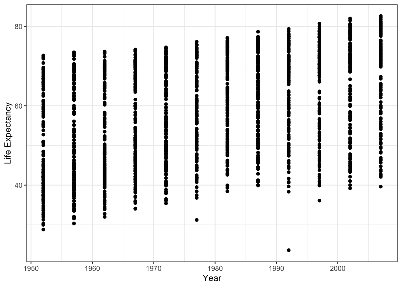 We can add a fitted line
ggplot(data = gapminder, aes(x = year, y = lifeExp)) +
geom_point() +
geom_smooth(method='loess', color = 'blue', se=FALSE) +
ylab('Life Expectancy') +
xlab('Year') +
theme_bw()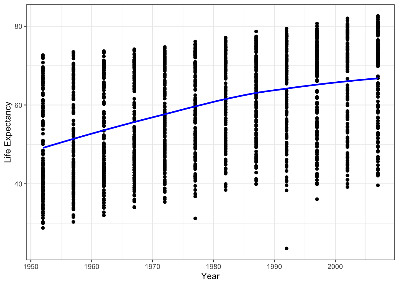 It looks like there is a positive relationship between year and life expectancy.
We can also fit a regression line using ggplot2
ggplot(data = gapminder, aes(x = year, y = lifeExp)) +
  geom_point() +
  geom_smooth(method='lm', color = 'blue', se=FALSE) +
  ylab('Life Expectancy') +
  xlab('Year') +
  theme_bw()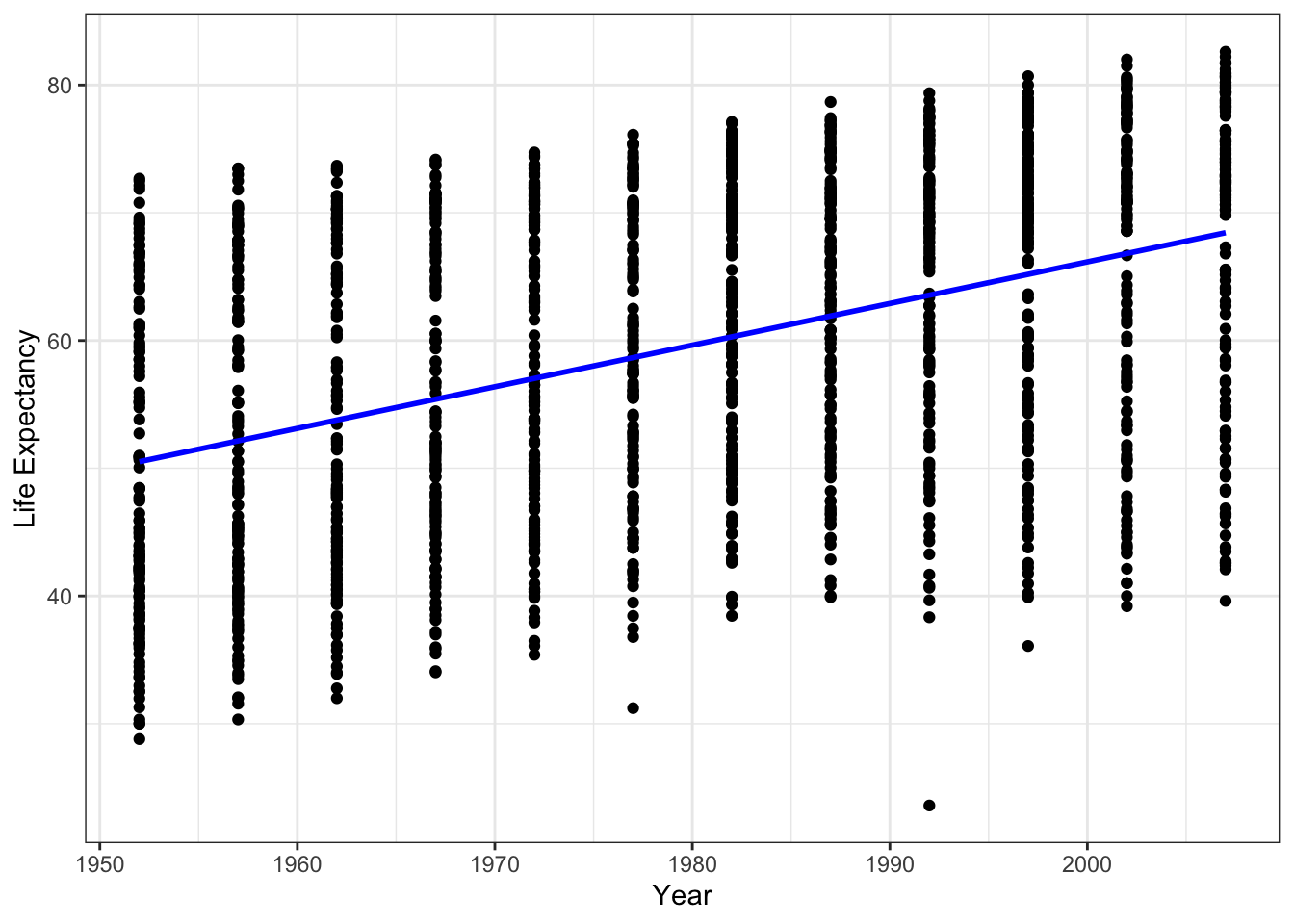
Now we will fit a linear model of the form:
\[y = \beta_0 + X \beta + \epsilon\]
where \(X\) is a 1706 X 4 matrix because there are 1706 observations (rows) and 4 variables. We can use the built in function lm() to run a linear model with life expectancy as our dependent variable. First, convert the population variable into a logged value.
gapminder$pop_log <- log(gapminder$pop) # make a logged population variableThen estimate the linear model \[\hat{y} = \hat{\beta}_0 + X\hat{\beta}\]
fit <- lm(lifeExp ~ year + country + pop_log + gdpPercap, data = gapminder)There are two functions we can use to get the fitted values
gapminder$yhat <- fit$fitted.values
gapminder$yhat <- fitted.values(fit)
We can check that the difference between our observed \(y\) and our \(\hat{y}\) is equal to our residuals.
r <- gapminder$lifeExp - gapminder$yhat
resid <- as.numeric(fit$residuals)
all.equal(r, resid)
## [1] "names for target but not for current"What is the predicted life expectancy for the United States in 1952 and in 2007?
US1952 <- gapminder %>% filter(country=='United States' & year==1952)
predict_US1952 <- predict(fit, newdata = US1952)

US2007 <- gapminder %>% filter(country=='United States' & year==2007)
predict_US2007 <- predict(fit, newdata = US2007)
predict_US1952;predict_US2007
## 1
## 65.42543## 1
## 81.42597We can also extract the variance-covariance matrix from our regression results
fit_vcov <- vcov(fit)
fit_vcov[1:3,1:3]
## (Intercept) year countryAlbania
## (Intercept) 336.2333899 -0.2375184633 13.06769134
## year -0.2375185 0.0001746932 -0.01129847
## countryAlbania 13.0676913 -0.0112984741 2.73849906#extract standard errors
se <- summary(fit)$coefficients[,2] # we want 2nd column
head(se^2,3)## (Intercept) year countryAlbania
## 3.362334e+02 1.746932e-04 2.738499e+00The variance-covariance matrix has the variance along the diagonal and we can see that it matches the variance.
Weighted Least Squares
We can show that the traditional OLS estimator is unbiased and linear. We are estimating the expectation of \(\hat{\beta}\) and assuming that there is constant error variance \(\epsilon_i \sim \mathcal{N}(0,\sigma^2)\). This model assumes \(\text{Var}(\epsilon_i) = \sigma^2\) for \(i = 1, \dots, n\). In other words, the variance of the residual \(\epsilon_i\) for each observation \(i\) is equal to \(\sigma^2\).
However, if we think there are nonconstant error variances \(\epsilon_i \sim \mathcal{N}(0, \sigma_{i}^2)\), we can use Weighted-least squares (WLS) as an alternative estimation method. Here we assume \(\text{Var}(\epsilon_i) = \frac{\sigma^2}{w_i}\) where the weights \(w_1, \dots w_n\) are known positive constants.
General Weighted Least Squares Solution
Let \(W\) be a diagonal matrix with diagonal elements equal to \(w_1, \dots w_n\).
\[ W = \begin{bmatrix} w_{1} & 0 & 0 \\ 0 & \ddots & 0\\ 0 & 0 & w_{n} \end{bmatrix} \] Weighted residual sum of squares \[S_w(\beta) = \sum_{i=1}^n w_i(y_i - x_{i}^t \beta)^2 = (Y - X\beta)^t W (Y-X\beta)\] WLS estimates \(\beta\) by minimizing the weighted sum of squares. The general solution is: \[\hat{\beta} = (X^t W X)^{-1}X^t WY\]
The weights
To use WLS we need to know the weights.
- We may have a probabilistic model in mind for the weights where \(\text{Var}(Y|X=x_i)\). For example we may think that the errors are proportional to a specific explanatory variable \(x_i\). Then we could use the reciprocal of this to estimate the weights: \(w_i = 1/x_i\).
For example let’s simulate data from a Poisson distribution.
set.seed(12345)
x <- rpois(100, lambda = 2)
y <- 3 + 4*x + rnorm(100, sd=2*x)
ggplot(data = data.frame(x,y),aes(x=x,y=y)) +
  geom_point() +
  geom_smooth(method=lm,se=FALSE) +
  theme_bw()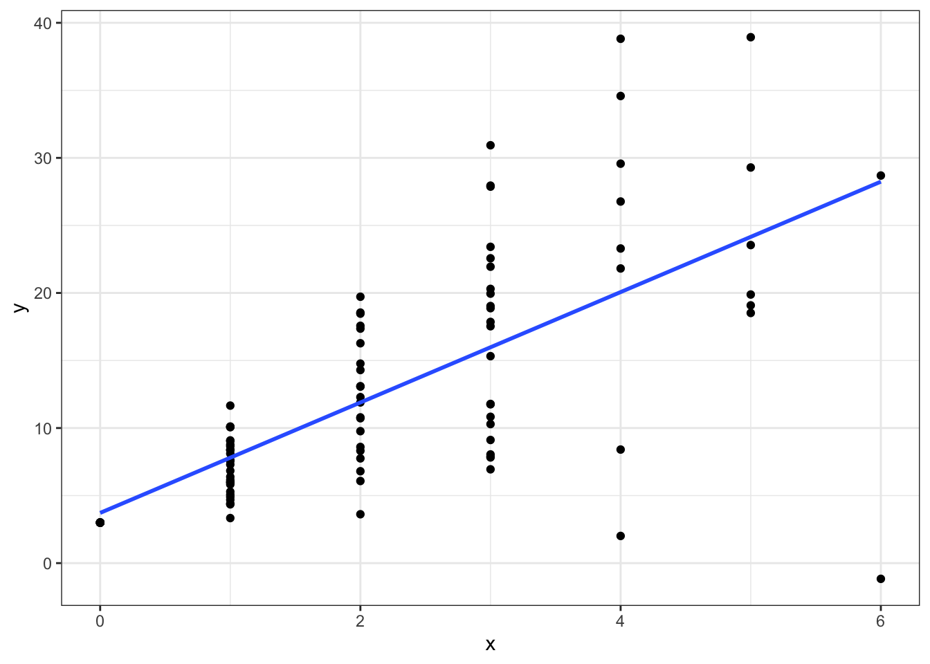
Notice how the variance in \(y\) gets larger as \(x\) gets larger. Now if we estimate a non-weighted linear regression:
fit_lm <- lm(y ~ x)
summary(fit_lm)
##
## Call:
## lm(formula = y ~ x)
##
## Residuals:
## Min 1Q Median 3Q Max
## -29.4022 -2.9553 -0.7186 2.5219 18.7514
##
## Coefficients:
## Estimate Std. Error t value Pr(>|t|)
## (Intercept) 3.7186 1.1052 3.365 0.0011 **
## x 4.0867 0.4305 9.492 1.53e-15 ***
## ---
## Signif. codes: 0 '***' 0.001 '**' 0.01 '*' 0.05 '.' 0.1 ' ' 1
##
## Residual standard error: 6.417 on 98 degrees of freedom
## Multiple R-squared: 0.479, Adjusted R-squared: 0.4737
## F-statistic: 90.11 on 1 and 98 DF, p-value: 1.53e-15Our \(\hat{\beta}\) estimate is 4.087 which is close to 4.
Now let’s estimate using WLS:
w <- 1/x #note there are 100 weights, one for each observation
w[w=='Inf'] <- 0 #fix any weights that occurred because 1/0 doesn't exist
fit_wls <- lm(y ~ x, weights = w)
summary(fit_wls)
##
## Call:
## lm(formula = y ~ x, weights = w)
##
## Weighted Residuals:
## Min 1Q Median 3Q Max
## -12.492 -2.343 0.000 1.756 9.080
##
## Coefficients:
## Estimate Std. Error t value Pr(>|t|)
## (Intercept) 3.1001 1.0529 2.944 0.00419 **
## x 4.3894 0.5065 8.666 2.79e-13 ***
## ---
## Signif. codes: 0 '***' 0.001 '**' 0.01 '*' 0.05 '.' 0.1 ' ' 1
##
## Residual standard error: 3.793 on 84 degrees of freedom
## Multiple R-squared: 0.472, Adjusted R-squared: 0.4657
## F-statistic: 75.1 on 1 and 84 DF, p-value: 2.791e-13Again, 4.389 is close to the true value of 4. If we look at a plot we can see that the weighted line in blue is above the red line as \(x\) gets larger. This is because the variance is getting larger and the WLS is downweighting these observations.
ggplot(data = data.frame(x,y),aes(x=x,y=y)) +
  geom_point() +
  geom_smooth(method=lm,se=FALSE,color='red') +
  geom_smooth(method=lm,aes(weight=w),color='blue',se=FALSE) +
  theme_bw()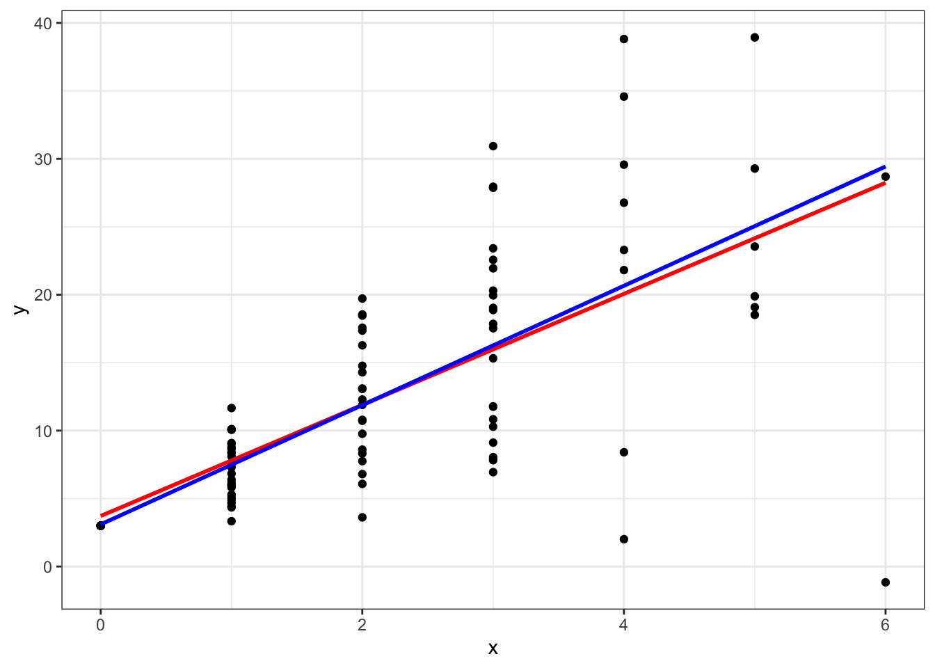
- Usually we do not know the weights nor the structure of \(W\) so we will first estimate the OLS regression.
Simulate data with non-constant errors:
set.seed(12345)
scalar <- 2
x <- rep(1:100,2)
sigma2 <- x^scalar
eps <- rnorm(x,mean=0,sd=sqrt(sigma2))
beta0 <- 3
beta1 <- 1
y <- beta0+beta1*x + eps
# fit linear model
fit_lm <- lm(y ~ x)
resid <- summary(fit_lm)$residuals
yhat <- fit_lm$fitted.values
# plot the residuals compared to x variable
ggplot(data.frame(x,resid),aes(x = x, y = resid)) +
  geom_point() +
  geom_hline(yintercept=0,color='green',linetype='dashed') +
  theme_bw()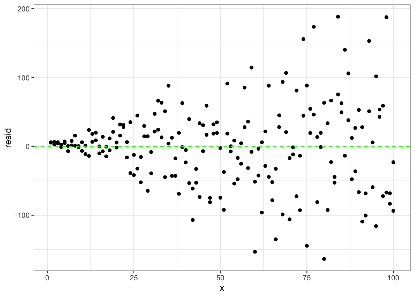
Looking at the plot of residuals compared to x values we see that as x gets larger so do the residuals.
There are different ways to calculate the weights using residuals. Here we are going to do the following steps:
- regress the residuals on the fitted values from the OLS model
- extract the fitted values from this regression
- use these fitted values squared as estimates of \(\sigma_{i}^2\) therefore we can estimate the weights as 1 over the square of the fitted values (\(w_i = 1/\sigma_{i}^2\))
# regress residuals on fitted values
fit_resid_yhat <- lm(abs(resid) ~ yhat)
# take fitted value of these
fitted <- fit_resid_yhat$fitted.values
w <- 1/(fitted^2)
fit_wls <- lm(y ~ x, weights = w)
htmlreg(list(fit_lm,fit_wls),custom.model.names = c("OLS","WLS"),doctype = F)| OLS | WLS | |
|---|---|---|
| (Intercept) | -2.60 | 1.82 |
| (8.50) | (2.26) | |
| x | 1.30*** | 1.20*** |
| (0.15) | (0.10) | |
| R2 | 0.29 | 0.44 |
| Adj. R2 | 0.28 | 0.43 |
| Num. obs. | 200 | 200 |
| ***p < 0.001; **p < 0.01; *p < 0.05 | ||
Both models estimate \(\beta_1\) pretty well. However, we’ve simulated the data with intercept equal to 3 but we see that the OLS estimate of the intercept is -2.6 while the WLS estimate of the intercept is closer at 1.82. Also note the big decrease in root mean squared error (RMSE) in the WLS model.
Plot both:
ggplot(data = data.frame(x,y),aes(x=x,y=y)) +
  geom_point() +
  geom_smooth(method=lm,se=FALSE,color='red') +
  geom_smooth(method=lm,aes(weight=w),color='blue',se=FALSE) +
  theme_bw()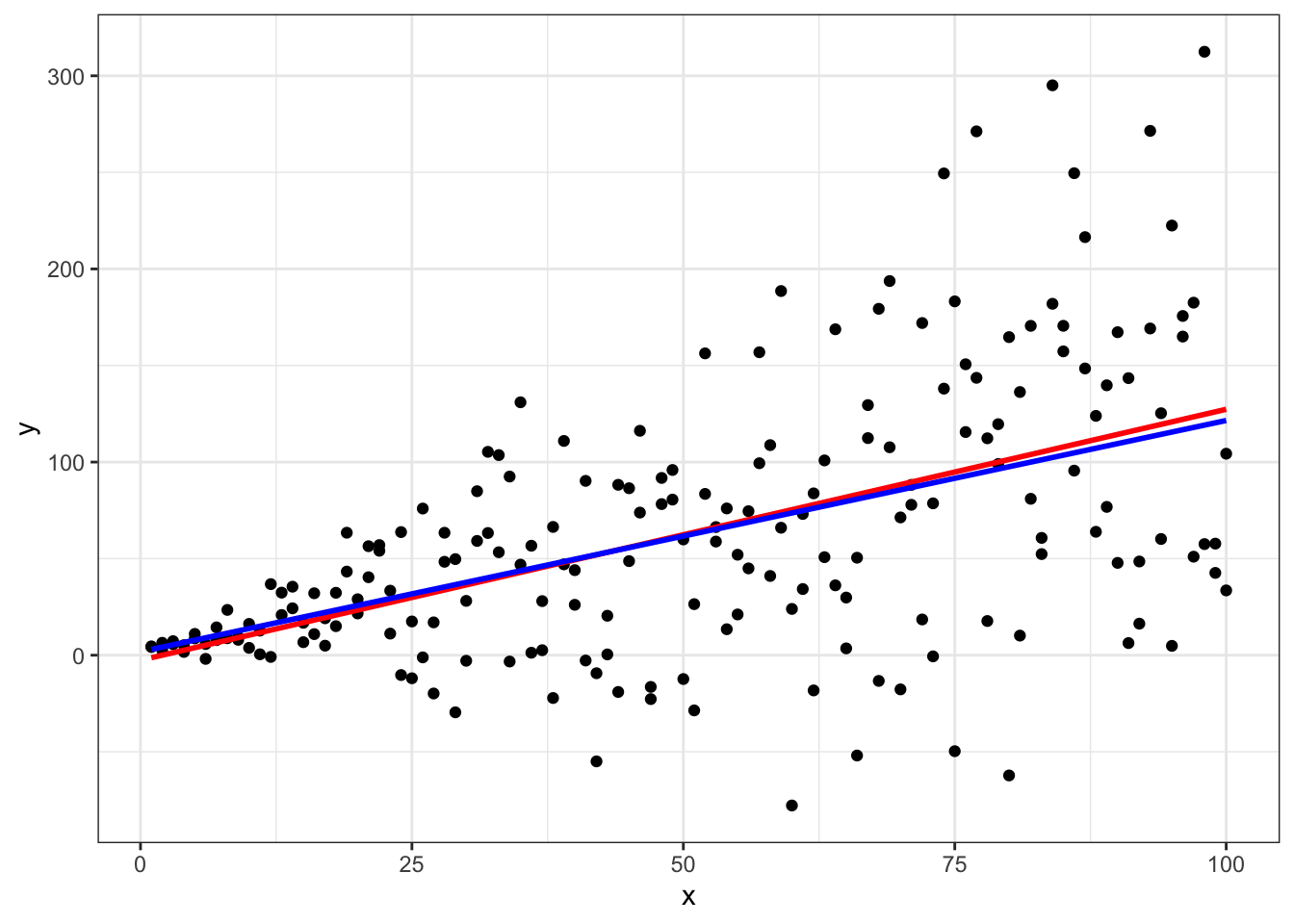
Again, we see that the WLS shifts slightly compared to OLS in order to down weight observations with extreme variances.
Note, that there are different ways to estimate the residuals. We can do it as in part 1 as the reciprocal of a specific predictor. Alternatively, the variances may be close to constant within specific subsets of a predictor. Or we might first estimate the OLS model and then use the residuals to help us estimate weights.